
Forecast 12 weeks of cinnamon export sales for 13,725 products across 91 countries, from 3.5 years of transactions. Sounds like a standard time-series exercise until you look at the data: for most products, most weeks are zero. This is not one forecasting problem but three stacked pathologies - and the whole project is shaped around treating each one as what it is.
- Intermittent demand: The signal has two parts classical methods conflate - when demand occurs and how much arrives. ARIMA and exponential smoothing assume continuous variation around a mean and collapse when the autocorrelation is dominated by zeros.
- Cold start: A product with five lifetime transactions has no usable per-series statistics; the only way forward is learning from related products.
- Hierarchy: Forecasts must stay coherent across total → region → country → product, but those levels have opposite character - the aggregate is smooth and easy, the disaggregate is sparse and hard.
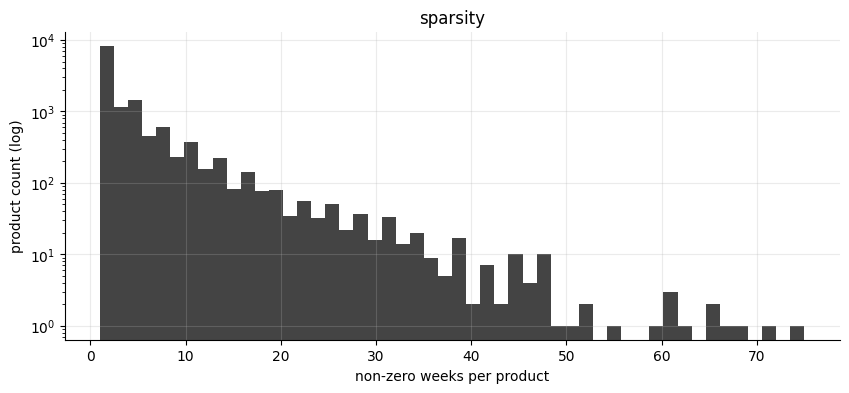
The problem in one picture: product count (log scale) vs non-zero weeks out of 187. The overwhelming majority of products sell in only a handful of weeks.
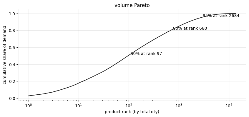
Meanwhile, volume is brutally concentrated: 97 products carry half of all demand; 680 carry 80%.
Why not one model - and why not an LSTM
The key structural fact of hierarchical intermittent data: aggregating sparse series produces dense, well-behaved ones. Different levels of the same hierarchy deserve different methods - which is why the design segments products first (ABC by volume, XYZ by demand variability) and routes each segment to the model suited to it, rather than forcing one model to cover everything.
The fashionable alternative - throw a neural sequence model at it - was considered and rejected on four grounds: with ~3.5 years of mostly-zero weekly data there isn't the sample volume neural methods need (the M5 competition was won by LightGBM, not neural nets); an LSTM trained with MSE on intermittent data learns to predict zero everywhere, the locally-optimal answer most of the time; vanilla sequence models have no notion of "this product is similar to that one," which is the entire cold-start fix; and tree models give feature importance for free where neural nets need SHAP bolted on.
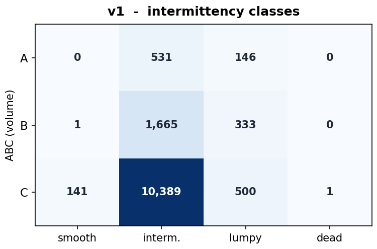
The segmentation that drives routing: volume class (A/B/C) against demand pattern. The 10,389-product C-intermittent cell is where naive models die.
The routing rule
- Retired (no sales in the last 52 weeks) → forecast zero. No model should be guessing here.
- Dense (12+ non-zero weeks, recently active) → a single global LightGBM trained across all products, with lags, rolling stats, calendar features, and holiday indicators for Sri Lanka plus the top 10 destination countries - cross-product learning is what rescues the cold-ish series.
- Sparse (2-11 non-zero weeks) → Croston's method, TSB variant. Croston decomposes an intermittent series into demand sizes and inter-arrival times - two far better-behaved series. TSB was chosen over the usual SBA correction deliberately: it updates demand probability every period rather than only when demand occurs, which is exactly the obsolescence-aware behavior needed for products that may be fading out.
- Nearly no history → flat historical mean rate. An honest fallback, labeled as such.
The data made its own case
Two discoveries during exploration changed the design. First, a single junk row claimed a quantity of 14,115,419 units with no date and no country - a reminder that cleaning rules (null-date drops, negative-quantity netting floored at zero) had to come before any modeling. Second, the raw region column turned out to be unreliable as geography: 19 countries appeared under multiple regions, with Sri Lanka filed under eight. The column encodes some business segmentation, not destination geography - so the hierarchy is built from a hand-made canonical country → region mapping instead, and the country level (which is clean) is trusted as-is.
Evaluation designed not to flatter
WAPE is the headline metric, always reported broken down by segment class - because a single blended number would hide the fact that sparse series are individually near-unforecastable. Validation is a three-way time split with three expanding-window walk-forward folds, and products that did not exist at the start of a fold are masked from it, so the models are never graded on questions the data could not have taught them.
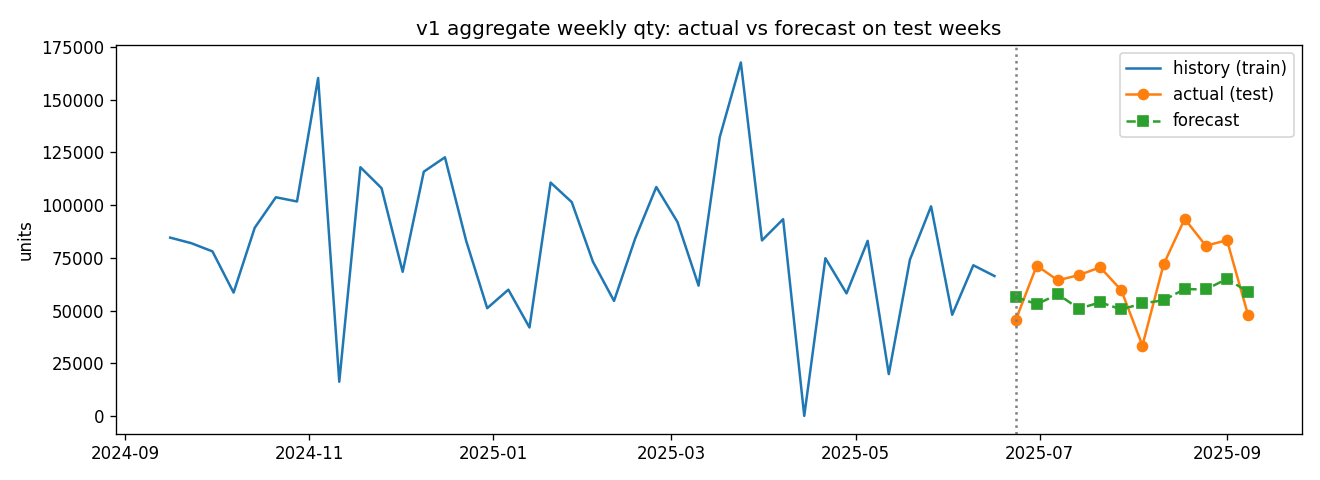
Held-out test: aggregate weekly actuals vs the reconciled forecast.
On the held-out test window, the shipped model blend reaches a total-level WAPE of 0.83 against 1.03 for seasonal naive and 0.94 for an 8-week moving average - roughly a 20% improvement over the standard benchmark, with the gains concentrated where the volume is (per-class results are reported alongside). The honest caveat stays in the report: at the individual sparse-product level, WAPE remains above 1.0 - no method meaningfully forecasts a series with three lifetime sales, and pretending otherwise is how forecasting projects mislead.
Deliverable
A 12-week forward forecast at product level with country-level drill-down, shipped as CSV - the country dimension coming essentially for free because 99.2% of products ship to a single country, so forecasting at the native (product, country, week) grain costs almost nothing extra.
For notebooks (a v0 baseline track and the shipped v1 track), utilities, outputs, and the full report, see the GitHub repository.